Tutorial: Organic Matter Degradation (Roden 2008)
This tutorial recreates the organic matter degradation experiment from Roden et al. (2008), demonstrating how to model sequential terminal electron acceptor processes.
Overview
In anoxic sediments, organic matter is degraded through a sequence of electron acceptors in order of decreasing energy yield:
- Nitrate reduction (NO₃⁻ → N₂)
- Iron reduction (Fe(III) → Fe(II))
- Sulfate reduction (SO₄²⁻ → H₂S)
- Methanogenesis (CO₂ → CH₄)
Each pathway is inhibited when a more favorable electron acceptor is available.
Step 1: Create the Batch Reactor
from porousmedialab.batch import Batch

# 40-day experiment with 1-day timestep
batch = Batch(tend=40, dt=1)
Step 2: Add Chemical Species
# Organic matter (electron donor)
batch.add_species(name='POC', init_conc=12e-3)  # mol/L

# Electron acceptors
batch.add_species(name='NO3', init_conc=1.5e-3)  # Nitrate
batch.add_species(name='Fe3', init_conc=20e-3)   # Fe(III)
batch.add_species(name='SO4', init_conc=1.7e-3)  # Sulfate

# Products
batch.add_species(name='CO2', init_conc=2e-3)    # Carbon dioxide
batch.add_species(name='Fe2', init_conc=0)       # Fe(II)
batch.add_species(name='CH4', init_conc=0)       # Methane
Step 3: Define Kinetic Constants
We use Michaelis-Menten kinetics with inhibition terms:
# Base degradation rate
batch.constants['k1'] = 0.1  # 1/day

# Half-saturation constants (inhibition thresholds)
batch.constants['Km_NO3'] = 0.001e-3   # Very low - NO3 inhibits others strongly
batch.constants['Km_Fe3'] = 2e-3       # Moderate
batch.constants['Km_SO4'] = 0.3e-4     # Low
Step 4: Define Rate Expressions
Each pathway is inhibited by all more favorable acceptors:
# Nitrate reduction - no inhibition
batch.rates['r_NO3'] = 'k1 * POC * NO3 / (Km_NO3 + NO3)'

# Iron reduction - inhibited by nitrate
batch.rates['r_Fe3'] = 'k1 * POC * Fe3 / (Km_Fe3 + Fe3) * Km_NO3 / (Km_NO3 + NO3)'

# Sulfate reduction - inhibited by nitrate and iron
batch.rates['r_SO4'] = 'k1 * POC * SO4 / (Km_SO4 + SO4) * Km_Fe3 / (Km_Fe3 + Fe3) * Km_NO3 / (Km_NO3 + NO3)'

# Methanogenesis - inhibited by all others
batch.rates['r_CH4'] = 'k1 * POC * Km_SO4 / (Km_SO4 + SO4) * Km_Fe3 / (Km_Fe3 + Fe3) * Km_NO3 / (Km_NO3 + NO3)'
Note the inhibition pattern: Each rate includes Km / (Km + Acceptor) terms for all more favorable acceptors. When the acceptor concentration is high, this term → 0, inhibiting the reaction.
Step 5: Set Mass Balance Equations (dcdt)
Apply stoichiometric coefficients:
# Organic matter consumption (sum of all pathways)
batch.dcdt['POC'] = '- r_NO3 - r_Fe3 - r_SO4 - r_CH4'

# Electron acceptors (stoichiometry from reaction equations)
batch.dcdt['NO3'] = '- 4/5 * r_NO3'      # 5 CH2O + 4 NO3 → ...
batch.dcdt['Fe3'] = '- 4 * r_Fe3'         # CH2O + 4 Fe(III) → ...
batch.dcdt['SO4'] = '- 1/2 * r_SO4'       # 2 CH2O + SO4 → ...

# Products
batch.dcdt['Fe2'] = '4 * r_Fe3'
batch.dcdt['CO2'] = 'r_NO3 + r_Fe3 + r_SO4 + 0.5 * r_CH4'
batch.dcdt['CH4'] = '1/2 * r_CH4'
Step 6: Run the Simulation
batch.solve()
Step 7: Visualize Results
import matplotlib.pyplot as plt

fig, ax1 = plt.subplots(figsize=(8, 5))
ax2 = ax1.twinx()

# Left axis: NO3, SO4, CH4
ax1.plot(batch.time, 1e3 * batch.NO3.concentration[0], label='NO₃')
ax1.plot(batch.time, 1e3 * batch.SO4.concentration[0], label='SO₄')
ax1.plot(batch.time, 1e3 * batch.CH4.concentration[0], label='CH₄')
ax1.set_ylabel('NO₃, SO₄, CH₄ [mM]')
ax1.set_ylim(0, 2.5)

# Right axis: Fe(II), CO2
ax2.plot(batch.time, 1e3 * batch.Fe2.concentration[0], 'C3', label='Fe(II)')
ax2.plot(batch.time, 1e3 * batch.CO2.concentration[0], 'C4', label='CO₂')
ax2.set_ylabel('Fe(II), CO₂ [mM]')
ax2.set_ylim(0, 25)

ax1.set_xlabel('Time [days]')
ax1.legend(loc='upper left')
ax2.legend(loc='upper right')
plt.show()
Results
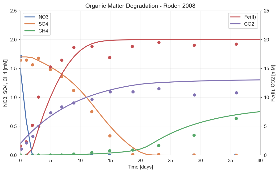
The simulation shows the characteristic sequential pattern:
- Days 0-2: NO₃ is rapidly consumed (blue line drops to zero)
- Days 2-15: Fe(III) reduction dominates, Fe(II) accumulates (orange)
- Days 10-25: SO₄ reduction begins as Fe(III) depletes (orange drops)
- Days 20+: Methanogenesis starts as SO₄ depletes (green rises)
CO₂ (purple) accumulates throughout as the product of all degradation pathways.
Key Takeaways
- Inhibition terms create the sequential pattern - each pathway waits for more favorable acceptors to deplete
- Michaelis-Menten kinetics provide smooth transitions between pathways
- Stoichiometric coefficients ensure mass balance
Complete Code
from porousmedialab.batch import Batch
import matplotlib.pyplot as plt

# Create batch
batch = Batch(tend=40, dt=1)

# Species
batch.add_species(name='POC', init_conc=12e-3)
batch.add_species(name='CO2', init_conc=2e-3)
batch.add_species(name='Fe2', init_conc=0)
batch.add_species(name='CH4', init_conc=0)
batch.add_species(name='NO3', init_conc=1.5e-3)
batch.add_species(name='Fe3', init_conc=20e-3)
batch.add_species(name='SO4', init_conc=1.7e-3)

# Constants
batch.constants['Km_NO3'] = 0.001e-3
batch.constants['Km_Fe3'] = 2e-3
batch.constants['Km_SO4'] = 0.3e-4
batch.constants['k1'] = 0.1

# Rates
batch.rates['r_NO3'] = 'k1 * POC * NO3 / (Km_NO3 + NO3)'
batch.rates['r_Fe3'] = 'k1 * POC * Fe3 / (Km_Fe3 + Fe3) * Km_NO3 / (Km_NO3 + NO3)'
batch.rates['r_SO4'] = 'k1 * POC * SO4 / (Km_SO4 + SO4) * Km_Fe3 / (Km_Fe3 + Fe3) * Km_NO3 / (Km_NO3 + NO3)'
batch.rates['r_CH4'] = 'k1 * POC * Km_SO4 / (Km_SO4 + SO4) * Km_Fe3 / (Km_Fe3 + Fe3) * Km_NO3 / (Km_NO3 + NO3)'

# Mass balance
batch.dcdt['POC'] = '- r_NO3 - r_Fe3 - r_SO4 - r_CH4'
batch.dcdt['NO3'] = '- 4/5 * r_NO3'
batch.dcdt['Fe3'] = '- 4 * r_Fe3'
batch.dcdt['Fe2'] = '4 * r_Fe3'
batch.dcdt['SO4'] = '- 1/2 * r_SO4'
batch.dcdt['CO2'] = 'r_NO3 + r_Fe3 + r_SO4 + 0.5 * r_CH4'
batch.dcdt['CH4'] = '1/2 * r_CH4'

# Solve and plot
batch.solve()
batch.plot_profiles()
Reference
Roden, E. E., & Jin, Q. (2011). Thermodynamics of microbial growth coupled to metabolism of glucose, ethanol, short-chain organic acids, and hydrogen. Applied and environmental microbiology, 77(5), 1907-1909.